Different Types of Linear Programming Problems

A few important linear programming problems are listed below:
1. Manufacturing problems.
2. Diet problems.
3. Transportation problems. In these problems, we determine a transportation schedule in order to find the cheapest way of transporting a product from plants/factories situated at different locations to different markets.

📌 Problem 1. Two godowns A and B have grain capacity of 100 quintals and 50 quintals respectively. They supply to 3 ration shops, D, E and F whose requirements are 60, 50 and 40 quintals respectively. The cost of transportation per quintal from the godowns to the shops are given in the following table:

Transportation cost per quintal (in $)
From/To	A	B
D	6	4
E	3	2
F	2.50	3

How should the supplies be transported in order that the transportation cost is minimum? What is the minimum cost?
✍ Solution:
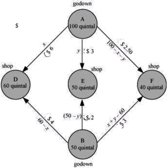
Let godown A supply x and y quintals of grain to the shops D and E respectively. Then, (100-x–y) will be supplied to shop F.
The requirement at shop D is 60 quintals since x quintals are transported from godown A. Therefore, the remaining (60-x) quintals will be transported from godown B. Similarly, (50-y) quintals and 40-(100-x–y)=(x+y-60) quintals will be transported from godown B to shop E and F respectively.
The given problem can be represented diagrammatically as follows. godown

x≥0, y≥0, and 100-x–y≥0
⇒ x≥0, y≥0, and x+y≤100.

60-x≥0, 50-y≥0 and x+y-60≥0
⇒x≤60, y≤50, and x+y≥60.
Total transportation cost z is given by,
z=6x+3y+2.5(100-x–y)+4(60-x)+2(50-y)+3(x+y-60)
=6x+3y+250-2.5x-2.5y+240-4x+100-2y+3x+3y-180
=2.5x+1.5y+410
The given problem can be formulated as
Minimize z=2.5x+1.5y+410…(1)
subject to the constraints,
x+y≤100…(2)
x≤60…(3)
y≤50…(4)
x+y≥60…(5)
x, y≥0…(6)
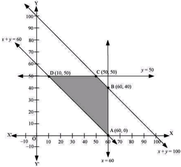
The feasible region determined by the system of constraints is as follows.

The corner points are A(60, 0), B(60, 40), C(50, 50), and D(10, 50).
The values of z at these corner points are as follows.

Corner point	z=7.5x+5y
A(60, 0)	560
B(60, 40)	620
C(50, 50)	610
D(10, 50)	510	→ Minimum

The minimum value of z is 510 at (10, 50).
Thus, the amount of grain transported from A to D, E, and F is 10 quintals, 50 quintals, and 40 quintals respectively and from B to D, E, and F is 50 quintals, 0 quintals, and 0 quintals respectively.

📌 Problem 2 (Transportation problem).
There are two factories located one at place P and the other at place Q. From these locations, a certain commodity is to be delivered to each of the three depots situated at A, B and C. The weekly requirements of the depots are respectively 5, 5 and 4 units of the commodity while the production capacity of the factories at P and Q are respectively 8 and 6 units. The cost of transportation per unit is given below:

From/To	Cost (in USD)
	A	B	C
P	160	100	150
Q	100	120	100

How many units should be transported from each factory to each depot in order that the transportation cost is minimum. What will be the minimum transportation cost?
✍ Solution:
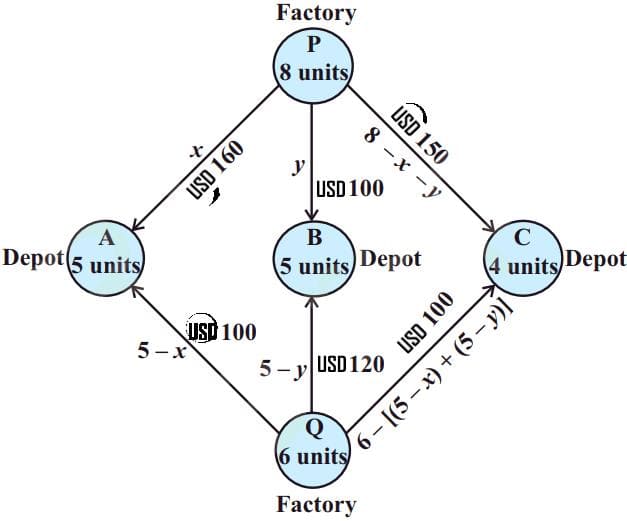
The problem can be explained diagrammatically as follows (Fig 1):

Let x units and y units of the commodity be transported from the factory at P to the depots at A and B respectively. Then (8-x–y) units will be transported to depot at C. (Why?)

[Fig 1]
Hence, we have x≥0, y≥0 and
8-x–y≥0→x+y≤8.

Now, the weekly requirement of the depot at A is 5 units of the commodity. Since x units are transported from the factory at P, the remaining (5-x) units need to be transported from the factory at Q. Obviously, 5-x≥0, i.e. x≤5.

Similarly, (5-y) and 6-(5-x+5-y)=x+y-4 units are to be transported from the factory at Q to the depots at B and C respectively.

Thus, 5-y≥0, x+y-4≥0
i.e. y≤5, x+y≥4

Total transportation cost Z is given by

Z=160x+100y+100(5-x)+120(5-y)+100(x+y-4)+150(8-x–y)
=10(x-7y+190).
Therefore, the problem reduces to minimise Z=10(x-7y+190) subject to the constraints:

x≥0, y≥0…(1)
x+y≤8…(2)
x≤5…(3)
y≤5…(4)
and x+y≥4…(5)

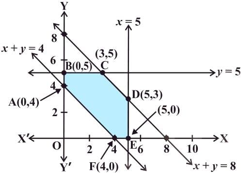
The shaded region ABC EF represented by the constraints (1) to (5) is the feasible region (Fig 2).

[Fig 2]

Observe that the feasible region is bounded. The coordinates of the corner points of the feasible region are (0, 4), (0, 5), (3, 5), (5, 3), (5, 0) and (4, 0). Let us evaluate Z at these points.

Corner Point	Z=10(x-7y+190)
(0, 4) (0, 5) (3, 5) (5, 3) (5, 0) (4, 0)	1620 1550 ← Minimum 1580 1740 1950 1940

From the table, we see that the minimum value of Z is 1550 at the point (0, 5).

Hence, the optimal transportation strategy will be to deliver 0, 5 and 3 units from the factory at P and 5, 0 and 1 units from the factory at Q to the depots at A, B and C respectively. Corresponding to this strategy, the transportation cost would be minimum, i.e., USD1,550.