The Quartile Common Formulae for Continuous or Discrete Distribution (Grouped Data)
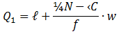
The median divides the distribution in two equal parts. The distribution can similarly be divided in more equal parts (four, five, six etc.). Quartiles for a continuous distribution is given by

Where, N= total frequency
ℓ= lower boundary of the first quartile class
f= frequency of the first quartile class
‹C= the cumulative frequency corresponding to
the class just before the first quartile class
w= the length of the first quartile class
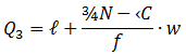
Similarly,

where symbols have the same meaning as above only taking third quartile in place of first quartile.

Frequency Distribution
The organization of a set of data in a table showing the distribution of the data into classes or groups together with the number of observations in each class or group is called frequency distribution. The number of observations falling in a particular class is referred to as the class frequency or simply frequency and is denoted by f.

Class Limits
The class limits are defined as the number of values of the variables which describe the classes; the smaller number is the lower class limit and the larger number is the upper class limit.

Class Boundaries
The class boundaries are the precise numbers which separate one class from another. A class boundary is located midway between the upper limit of a class and the lower limit of the next higher class.

Class Mark
A class mark, also called class midpoint, is the number which divides each class into two equal parts. It is obtained by dividing either the sum of the upper and lower class limits, or the sum of the upper and lower class boundaries by 2.

Class Width or Interval
The width or interval of a class is equal to the difference between the class boundaries. It is also obtained by finding the difference between two successive lower class limits.

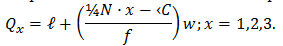
Quartiles
Using the same method of calculation as in the Median,
we can get Q₁ and Q₃ equation as follows:

Example 1: Based on the grouped data belo w, find the Interquartile Range

Time to travel to work	Frequency
1-10 11-20 21-30 31-40 41-50	8 14 12 9 7

Solution:
1st Step: Construct the cumulative frequency distribution

Time to travel to work	Frequency	Cumulative Frequency
1-10 11-20 21-30 31-40 41-50	8 14 12 9 7	8 22 34 43 50

2nd Step: Determine the Q₁ and Q₃.
Class Q₁=¼N=¼⋅50=12.5
Class Q₁ is the 2nd class
Therefore,

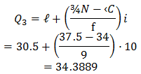
Class Q₁=¾N=¾⋅50=37.5
Class Q₃ is the 4th class
Therefore,

Interquartile Range
IQR=Q₃–Q₁
calculate the IQ
IQR=Q₃–Q₁=34.3889-13.7143=20.6746

Example 2:
Find the the quartiles Q₁, Q₂, and Q₃ of the following data.

Columns Load	Freqency (fi)
50-69	3
70-89	7
90-109	4
110-129	4
130-149	9

Solution:
step 1) Find each cumulative frequency and each real interval.

step 2) Find the point of first quartile.
q₁=¼N=¼⋅27= 6.75
The interval where the first quartile lies has the cumulative frequency of 10.

ℓ= the lower boundary of relevant quartile class =69.5
N= total frequency
‹C= the cumulative frequency of the previous interval of relevant quartile class =3
f= the frequency of relevant quartile class =7
w= the length of the real interval =20

step 3) Find the point of second quartile.

The interval where the second quartile lies has the cumulative frequency of 14.

step 4) Find the point of third quartile..
q₃=¾N=¾⋅27= 20.25
The interval where the third quartile lies has the cumulative frequency of 27.

Example 3: Calculation of Quartile Deviation (Q.D.) for a frequency distribution.
For the following distribution of marks scored by a class of 40 students, calculate the Range and Q.D.

Class intervals	Number of students (f)
0<x≤10 10<x≤20 20<x≤40 40<x≤60 60<x≤90	5 8 16 7 4
sum:	40

Range is just the difference between the upper limit of the highest class and the lower limit of the lowest class. So Range is 90–0=90. For Q.D., first calculate cumulative frequencies as follows:

Class intervals	Frequencies (f)	Cumulative Frequencies (c.f.)
0<x≤10 10<x≤20 20<x≤40 40<x≤60 60<x≤90	5 8 16 7 4	5 13 29 36 40
sum:	N=40

Q₁ is the size of ¼Nth value in a continuous series. Thus it is the size of the 10th value. The class containing the 10th value is 10–20. Hence Q₁ lies in class 10–20. No w, to calculate the exact value of Q₁, the following formula is used:

Where ℓ=10 (lower boundary of the relevant Quartile class)
‹C = 5 (value of c.f. for the class preceding the Quartile class)
w=10 (interval of the Quartile class), and
f=8 (frequency of the Quartile class) Thus,

Similarly, Q₃ is the size of ¾Nth value; i.e., 30th value, which lies in class 40–60. No w using the formula for Q₃, its value can be calculated as follows:

In individual and discrete series, Q₁ is the size of ¼(N+1)th value, but in a continuous distribution, it is the size of ¼N th value. Similarly, for Q₃ and median also, n is used in place of N+1.

If the entire group is divided into two equal halves and the median calculated for each half, you will have the median of better students and the median of weak students. These medians differ from the median of the entire group by 13.31 on an average. Similarly, suppose you have data about incomes of people of a town. Median income of all people can be calculated. No w if all people are divided into two equal groups of rich and poor, medians of both groups can be calculated. Quartile Deviation will tell you the average difference between medians of these two groups belonging to rich and poor, from the median of the entire group.

Quartile Deviation can generally be calculated for open-ended distributions and is not unduly affected by extreme values.

Other measures of variation:
The variance and standard deviation are regarded as the best and the most powerful mea- sures of dispersion. One of the dra w backs with these measures of dispersion is that they are influenced by extreme observations. Thus, many statisticians think that if the median is used (instead of the mean) as a measure of central tendency because of the presence of the outliers, then some other measures of dispersion, namely the interquartile range or the quartile deviation, should be used to describe the variability.

Interquartile range:
The interquartile range is the difference between the third quartile and the first quartile. That is

Interquartile range =Q₃–Q₁.

Quartile deviation:
The quartile deviation is the half of the difference between the third quartile and the first quartile. That is

Quartile deviation =½(Q₃–Q₁).

Example 4:
Find the interquartile range and the quartile deviation for the given data in the table below:

Scores	Frequency
50-59 60-69 70-79 80-89 90-99	8 22 12 5 3

Solution:

sum:

Scores	Class boundary	f	c.f
50-59 60-69 70-79 80-89 90-99	49.5-59.5 59.5-69.5 69.5-79.5 79.5-89.5 89.5-99.5	8 22 12 5 3	8 30 42 47 50
		N=50

Calculation of Q₁:

Q₁=¼Nth observation
=12.5th observation, which lies in the class 59.5-69.5.
⇒Q₁ class=59.5—69.5. Therefore,

Calculation of Q₃:
Q₃=¾N th observation
=37.5th observation, which lies in the class 69.5—79.5.
⇒Q₃ class = 69.5—79.5. Therefore,

Hence,
Interquartile range =Q₃–Q₁
=75.8-61.5=14.3
and
Quartile deviation =½(Q₃–Q₁)
=½(75.8-61.5)=7.15
Let’s read post Calculation of Deciles for Grouped Data.